
During the 2016 General Election, the Clinton campaign reportedly spent almost twice as much money as the Trump campaign, and lost. How was this outcome possible? Campaign spending is supposed to translate into votes. Of course, Clinton did win the popular vote, by several million votes in fact. Her margin of defeat in the Electoral College was, by contrast, fairly thin. Indeed, the combined margin of victory for Trump in Pennsylvania, Michigan, and Wisconsin was a mere 77,759 votes. If Clinton could have persuaded 1% of voters in each state, she would have won. The drastic inefficiency in where Clinton votes were allocated raised questions about whether her campaign had targeted its spending effectively. According to The Washington Post, in the last few weeks of the election, the Clinton campaign aired more ads in “Omaha than the states of Michigan and Wisconsin combined.”
Mismanagement is a tempting explanation for what happened. Yet, to accept the explanation that Clinton spent badly, we need to believe that effective campaign spending would have made up the difference. This proposition may seem uncontroversial. Pundits and politicians often attest that campaign spending usually makes a big difference. The Supreme Court assumes that campaign spending effects outcomes when it allows Congress and the FEC to regulate campaign finance. Surely, campaign spending can and usually does affect outcomes in a significant way.
Surprisingly, there is an active debate among political scientists about whether ad spending determines election outcomes in any sense. Indeed, a recent meta-analysis by Joshua Kalla and David Broockman of nearly fifty electoral field experiments found that “the best estimate for the persuasive effects of campaign contact and advertising… is zero” (Kalla and Broockman, 2017).
Such experimental evidence surely makes it reasonable to doubt advertising effects of Presidential campaigns are all they’re cracked up to be. However, presidential campaign spending occurs on a vastly different economic scale than what field experiments have analyzed. That difference of scale could matter. The issue is easier to understand by analogy to the medical context. We know that a typical dose of ibuprofen decreases headaches. But no matter how many double-blind studies we run, if we always test with just a few milligrams of ibuprofen, we are unlikely to ever observe the effect of the typical 200 milligram pill. By analogy, maybe the dosage in field experiments is just too small.
Yet upping the dose on campaign experiments is logistically challenging. In order to evaluate campaign effects “at scale,” researchers generally use observational evidence. Observational data introduce many difficulties of their own. How do we know who saw the ads and who did not? Are we sure that those that did see the ads were not different from those that did not for unrelated reasons? These are tough problems.
Recently, Guillaume Pouliot and I have been working on a new, causally credible approach to estimating the persuasive effects of advertising. One of our data sources, the USC’s Daybreak Election Poll, is a 17-week panel of many thousands of participants. For our purposes, this panel differs from previous surveys in two key respects. First, the USC survey tracks the same set of individuals over time. Most, but not all, election surveys use a “rolling” cross-section so that the participants are constantly changing; it’s impossible to tell what’s happening to any particular individual. But if ads do have a persuasive effect, it has to persuade particular individuals to change their minds at particular points in time.
The second significant respect in which this survey differs from previous data sources is that 17-weeks is a lot of observations for each individual. Previous studies that track the same individuals over time have typically only done so during two periods, before and after the election. So in terms of unpacking attitudes, our data source is not only bigger, it is also more granular than anything the observational literature has used.
Our other data source is a dynamic spending database built from scraping TV station’s “public files.” When a broadcaster sells ad time to a political campaign, the Federal Communications Commission (FCC) requires the station to keep the invoices. In the old days, which in this case means prior to 2014, broadcasters would keep copies locally. 2016 was the first Presidential campaign cycle during which all TV stations were required to post their records electronically on the FCC’s website. The Center for Responsive Politics has been working on organizing and cataloguing this data, and we worked with them to identify all the invoices for ads that individuals in the USC study could have received.
These invoices tell us exactly where and when spending occurred. It is likely that the data we obtain from these methods are more detailed than what campaigns themselves reviewed and analyzed, since campaigns typically delegate the ad placement tasks to more specialized marketing firms. The downside is that, with thousands of different TV stations across the country, this information is presented in different ways and sometimes the information is hard for a computer to read. Cleaning this data is a major task, and it’s what my collaborator and I are presently working on.
Even so, the results that we have are interesting. Figure 1 shows how strongly each member of the USC study was leaning between Clinton and Trump over time; each person is represented by a line of color on the spectrum between blue and red. Apparently, over half of the nationally representative sample exhibited almost no change in their views between July and November of 2016. When there is change in a person’s views, it is usually between varying degrees of certainty. There are very few instances of apparent “conversion.” Again, this observation makes it unlikely that the effect of campaign spending is substantial.
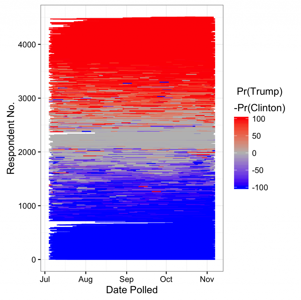
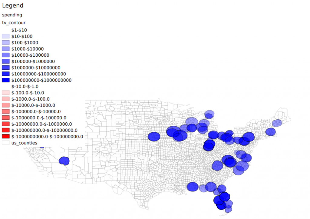
On the spending side, our conclusions are more tentative as we’ve only been able to gather data from about 50% of the invoices we have. Still, Figure 2 shows the aggregate general election spending in TV stations that members of the USC study could have observed. So far, it appears that Clinton outspent Trump to the tune of millions of dollars essentially everywhere, including Michigan, Wisconsin, and Pennsylvania. Much of this spending advantage was amassed in the first few weeks of the general election campaign, however. At the end the Clinton spending advantage was smaller, and in some places Trump had the advantage. These spending patterns have implications for how we interpret Figure 1. If campaign spending had a substantial effect, we should expect the left and right side of the graph to look rather different, since the spending environment was different in these two periods.
Coming to firm conclusions about the effect of ad spending is important. If ad spending does little to change vote margins, then candidates should run their campaigns differently. Donors who collectively give billions of dollars every election cycle could allocate their money differently. Good government reformers might shift their attention to other issues that might make a bigger difference, for example policies to change how states draw their legislative districts. On the other hand, if ad spending does change minds, it suggests redoubling our efforts at ensuring the fairness and transparency of election financing. Which position is better on the basis of our research? While it is still too early to say for sure, at this juncture we consider the evidence for persuasive effects of ad spending to be quite weak. Either Presidential campaign ads do not buy votes, or if they do, the price is so high that the campaigns themselves are not spending at a sufficiently high level to make a difference.
You must be logged in to post a comment.